DSP | Theory | Linear Systems

What is a system?

A system is a process that produces an output signal in response to an input signal. Thus, a system may itself be a composition of multiple systems.

Systems are described mathematically using a signal naming convention, whereby;

continuous signals are denoted using parentheses - x(t)
discrete signals are denoted using square brackets - x[t]
signals in the time domain are denoted using lowercase letters - x(t)
signals in the frequency domain are denoted using uppercase letters - X(f)

Thus, a discrete signal in the frequency domain might be Y[f].

Properties of Linear Systems

Linear Systems exhibit numerous qualities which make them very easy to work with, including;

Homogeneity

Any change in amplitude of an input signal will result in a calculable change in amplitude of the output signal.

Thus, if an input of x[n] results in y[n], then 2x[n] would result in 2y[n].

Additivity

Signals can be added together without interacting. Thus;

x₁[n] -> y₁[n]
x₂[n] -> y₂[n]
x₁[n] + x₂[n] -> y₁[n] + y₂[n]

Shift Invariance

A shift in the input signal causes an identical shift in the output signal, where;

x[n] -> y[n]
x[n + s] -> y[n + s]

Superposition

The response of a linear system to a sum of signals is the sum of the responses to each individual input signal. Therefore, if an input containing three signals were passed through a linear system, the output would be the same as if each signal were passed in individually, then combined at the output.

Impulse Decomposition

Impulse decomposition breaks up an n samples signal into n component signals, each containing n samples. Each of those component signals contains one point from the original signal, with all other values set to zero. The single non-zero point is, therefore, the impulse.

The aim of impulse decomposition is to enable the analysis of each sample, one at a time. Since linear systems are predictable, the output can therefore be calculated for any given input.

Step Decomposition

Step decomposition breaks up an n samples signal similarly to impulse decomposition, but arranges them as steps. This means that all samples proceding the focus sample are set to the same value, while preceding samples are zero as before.

Step decomposition characterizes signals by the difference between adjacent samples.

Unit Impulse

The unit impulse function is a fundamental function in DSP. The symbol of a unit impulse function is the Greek delta δ. Here, δ(n) = 1 if n = 0, and 0 everywhere else.

Questions

This section contains my own answers to questions. They may or may not be correct.

Impulse Function and Digital Signals

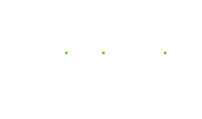
(a) Draw three impulse function, `δ[n - v]` for values of `v = 0`, `v = 5` and `v = -3`

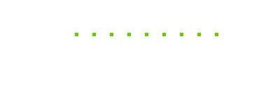
(b) Given a function `g(n) = 5` draw `g(k)δ[n - k]` for values of `-5 < k < 5`

(c) If a continuous sine wave is defined as `x(t) = a sin(t2πf)` define the digital version using `n` for the samples and `T_s` seconds for the sample interval.

x[n] = a sin(n2π(f/f_s))

(d) State the sample frequency of this digitised sine wave (remember to include units).

f_s

(e) If the frequency of the sine wave is `8000Hz`, what is the period (remember to include units)?

1/8000 = 125e-6 = 125µs

Linear Time Invariant Systems and Digital Convolution

(a) What is the Princsple of Superposition and why is it useful?

Superposition is the means by which the sum of unique output signals through a system is equivelent to the sum of an output of the same signals from a system. Thus, if you feed all signals combined, or feed signals individually and combine at the output, the result is the same.

(b) Draw the system diagram using time delays, addition and multiplication for a moving average filter `y[n] = (x[n] + x[n-1] + x[n-2] + x[n-3] + x[n-4]) / 5`

(c) Calculate the impulse response of this moving average filter (5 stage) showing all steps.

x[n] = [1,0,0,0,0], h[n] = 1/5 x[n-1] = [0,1,0,0,0], h[n-1] = 1/5 x[n-2] = [0,0,1,0,0], h[n-2] = 1/5 x[n-3] = [0,0,0,1,0], h[n-3] = 1/5 x[n-4] = [0,0,0,0,1], h[n-4] = 1/5 h[n] = (1/5) when 0 ≤ n < 5 and 0 everywhere else

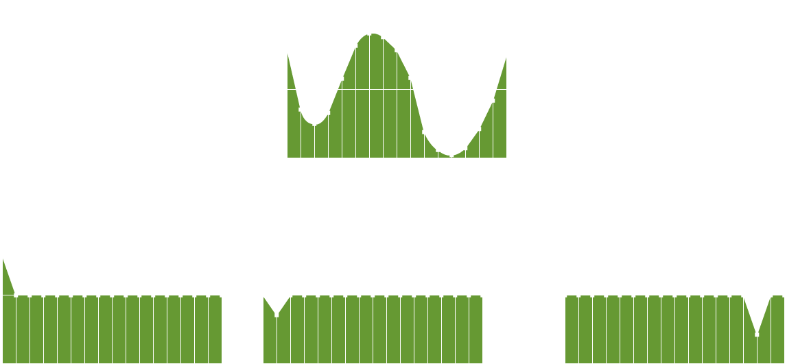
(d) Convolve, showing all calculation steps, this moving average filter with a unit step function `u[n] = {1 if n ≥ 0, 0 if n < 0}`

1/5 = h[0] 2/5 = h[0] + h[1] = (1/5) + (1/5) 3/5 = h[0] + h[1] + h[2] = (1/5) + (1/5) + (1/5) 4/5 = h[0] + h[1] + h[2] + h[3] = (1/5) + (1/5) + (1/5) + (1/5) 1 = h[0] + h[1] + h[2] + h[3] + h[4] = (1/5) + (1/5) + (1/5) + (1/5) + (1/5) 1 = h[0] + h[1] + h[2] + h[3] + h[4] + h[5] = (1/5) + (1/5) + (1/5) + (1/5) + (1/5) + 0 ...

(e) `y[n] = (1/4) (x[n+1] + x[n] + x[n-1] + x[n-2])` and `y[n] = (1/4) (x[n] + x[n-1] + x[n-2] + x[n-3])` are 4 term non-causal and causal moving average filters respectively. What does non-causal mean? (Explain in 1 sentence).

Non-causal typically refers to a convolution algorithm that is not dependent on future (+) signal values.

(f) The equations for these 4 term moving average filters are known as difference equations. Most differene equations for Linear Time Invariant (LTI) systems can be put into the following form. Place the 4 term moving average filters into this more general form.

Non-Causal

Causal

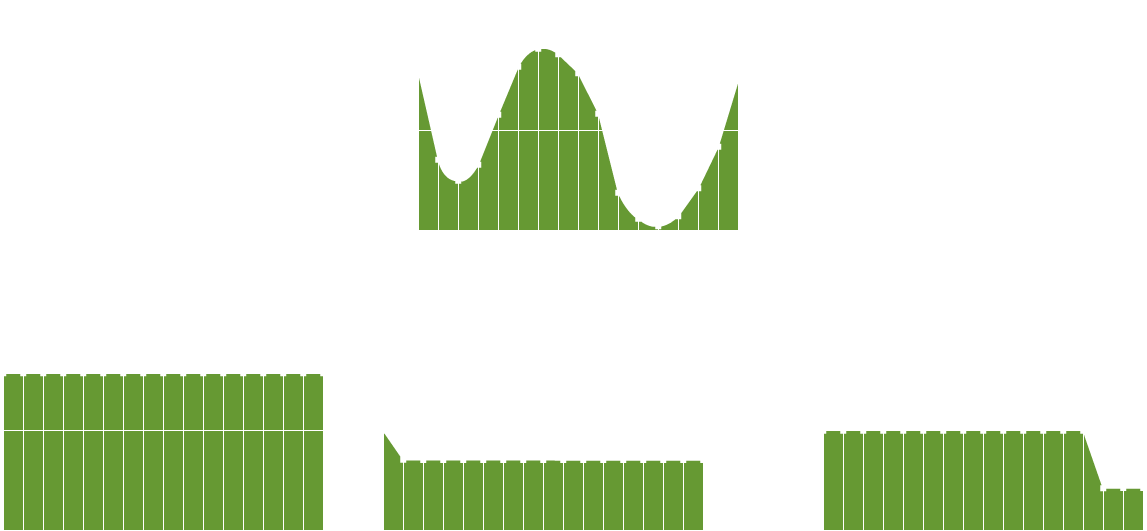
(g) Convolve a 2 term causal moving average filter y[n] with the following signal.

f[n] = 2 when n = 3, 0.5 when 0 ≤ n ≤ 2, 0.7 when 4 ≤ n ≤ 7, 0 everywhere else

Show all essential working and steps.

Here, no values are given for input indicies less than zero, so we can outline causal only. Maximum value is 7 (+1 for 2 term impulse).

(n = 0) = (1/2)(0.5 + 0) = 0.25 (n = 1) = (1/2)(0.5 + 0.5) = 0.5 (n = 2) = (1/2)(0.5 + 0.5) = 0.5 (n = 3) = (1/2)(2 + 0.5) = 1.25 (n = 4) = (1/2)(0.7 + 2) = 1.35 (n = 5) = (1/2)(0.7 + 0.7) = 0.7 (n = 6) = (1/2)(0.7 + 0.7) = 0.7 (n = 7) = (1/2)(0.7 + 0.7) = 0.7 (n = 8) = (1/2)(0 + 0.7) = 0.35 (n = 9) = 0 ...

← Back to Digital Signal Processing