DSP | Theory | Convolution

Convolution is the mathematical operation of combining two signals to get a resulting signal. Typically, the two signals in question are the input signal and the impulse response.

Delta Function

The delta function is a normalised impulse response. Another way of describing it is as the unit impulse or the identity of convolution, much like 0 is the identity of addition and 1 is the identity of multiplication.

The delta function is denoted as δ[n], pronounced delta of n.

The result of the delta function is that the sample of n is one, while all other samples are zero.

Impulse Response

The impulse response is the signal produced as output when the delta function is provided as input to a system. Here, different systems will produce different impulse responses.

The impulse response is denoted as h[n], pronounced h of n.

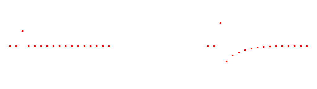
Any impulse can be represented as a shifted and scaled delta function. For example, x[n] = -1.5δ[n - 8] would result in;

which is essentially the delta function shifted right by 8 samples and multipled by 1.5.

In digital filter design, the impulse response is called the filter kernel, convolution kernel or simply the kernel. In image processing, however, it is termed point spread function.

Convolution Operation

The convolution operation is represented by an asterisk *. Thus, input * impulse_response = output.

Output Length

The output signal length will be equal to the input length plus the impulse response length minus 1.

y[n] = x[n] + h[n] - 1

Thus, an input with 8 samples and an impulse response of 6 signals will result in an output of 13 samples.

The Operation

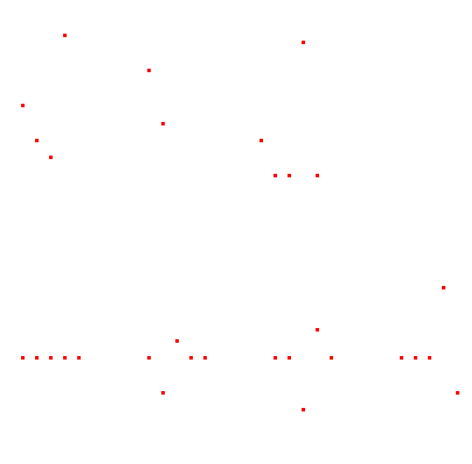
The input signal is decomposed into single sample components and each component is passed through the system. Each of those samples then contribute to a scaled and shifted version of the impulse response. The output components are then synthesized (combined) to produce the output signal.

Let’s take a simple example.

Input [0, -1, -1.5, 2] Σ Impulse Response [1, -0.5]

To convolute, we apply the scale from the impulse response to index n, shifted n places for each index up to x[n] - (h[n] - 1)

The equation, therefore, is;

where M is the number of samples in h[n] and j is merely an iterator.

With this knowledge, we can therefore identify the convoluted value of a sample using the equation as follows.

To determine y[3];

y[3] = x[2]h[n-2] + x[3]h[n-3]
     = x[2]h[3-2] + x[3]h[3-3]
     = x[2]h[1] + x[3]h[0]
     = (-1.5 x -0.5) + (2 x 1)
     = 0.75 + 2
     = 2.75

Delta Function Revisited

Note that the simplest impulse response is the delta function, so that;

x[n] * δ[n] = x[n]

where convoluting any signal with a delta function results in the exact same signal.

Delta Function Scaling

If you increate the amplitude of the delta function, then the resulting impulse response is amplified, while a decreased amplitude will attenuate;

x[n] * kδ[n] = kx[n]

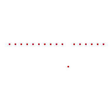
Delta Function Shifting

Shifting the delta function to the right produces a corresponding delay between the input signal and the output signal.

δ[n - s]

Shifting the delta function to the left produces a corresponding advance between the input signal and output signal.

δ[n + s]

Properties of Convolution

Convolution exhibits several mathematical properties, including;

Commutitive Property

x[n] * y[n] = y[n] * x[n]

Associative Property

(x[n] * y[n]) * z[n] = y[n] * (x[n] * z[n])

Distributive Property

(x[n] * y[n]) + (x[n] * z[n]) = x[n] * (y[n] + z[n])

← Back to Digital Signal Processing