DSP | Filters | Biquadratic Digital Filter
Calculators Theory Z-Domain Filters
Biquadratic PZ Placement Butterworth Chebyshev Prototypes IIR Filter
← Back to Digital Signal Processing
The figure below represents a biquadratic digital filter in state-variable realisation form.
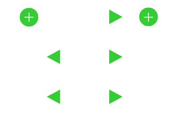
The values of the multipliers are as follows;
\[a = 0.37, b = -0.02, c = 0.16, d = -0.5, e = 0.06\]Time Domain Equation
Determine the time domain equations that raise the input \(x[n]\) to the intermediate system variable \(w[n]\) and the output \(y[n]\) and complete the following;
\[w[n] = x[n] + A \times w[n-1] + B \times w[n-2]\] \[y[n] = C \times w[n] + D \times w[n-1] + E \times w[n-2]\]Working down the filter, we can see the unit delays occur from \(w[n]\) through to \(w[n-2]\). The values are therefore multiplied previously to the adder in the following order;
\[A = a, B = b, C = c, D = d, E = e\]Z-Domain Equation
Determine the z-domain equations that relate the input X(z) and the output Y(z) variables to the intermediate system W(z) variable, where;
\[X(z) = W(z)(1+A \times z^{-1} + B \times z^{-2})\] \[Y(z) = W(z)(C + D \times z^{-1} + E \times z^{-2})\]Well, we can simply convert the equations in the time domain to the z-domain, like so;
\[W(z) = X(z) + 0.37 \times W(z)z^{-1} - 0.02 \times W(z)z^{-2}\] \[Y(z) = 0.16 \times W(z) - 0.5 \times W(z)z^{-1} + 0.06 \times W(z)z^{-2}\]These can be rearranged, taking care to ensure inversion of operators where necessary;
\[X(z) = W(z) - 0.37 \times W(z)z^{-1} + 0.02 \times W(z)z^{-2}\] \[Y(z) = 0.16 \times W(z) -0.5 \times W(z)z^{-1} + 0.06 \times W(z)z^{-2}\]Factoring out \(W(z)\), we then have;
\[X(z) = W(z)(1 - 0.37z^{-1} + 0.02z^{-2})\] \[Y(z) = W(z)(0.16 - 0.5z^{-1} + 0.06z^{-2})\]Recalling that \(H(z) = Y(z)/X(z)\), we can divide the expressions;
\[H(z) = \frac{W(z)(0.16 - 0.5z^{-1} + 0.06z^{-2})}{W(z)(1 - 0.37z^{-1} + 0.02z^{-2})}\]Cancelling \(W(z)\);
\[H(z) = \frac{0.16 - 0.5z^{-1} + 0.06z^{-2}}{1 - 0.37z^{-1} + 0.02z^{-2}}\]MATLAB
a = 0.37; b = -0.02; c = 0.16; d = -0.5; e = 0.06;
% invert the values in the denominator
a = a * -1
b = b * -1
% the rest are intact
Z-Domain Transfer Function of Filter
From the above, we can determine the z-domain trasnfer function of the filter;
\[H(z) = \frac{K \times (z-z_{1})(z - z_{2})}{(z - p_{1})(z - p_{2})}\]Here, the values in the numerator are the zeros and the values in the denominator are the poles. We can determine these by finding the roots of the system.
First, multiply the result of the previous equation by \(z^{2}\) to give us a positive-z equation;
\[H(z) = \frac{0.16z^{2} - 0.5z + 0.06}{z^{2} - 0.37z + 0.02}\]To determine the zeros, we can bring out the \(0.16z\), but then we need to divide the remaining values by \(0.16\);
\[H(z) = \frac{0.16(z^{2} - 3.125z + 0.375)}{z^{2} - 0.37z + 0.02}\]Thus, the zeros are - in size order! - \(0.375\) and \(3.125\), while the multiplier is \(0.16\).
MATLAB (midway)
% bringing out c, we divide the other two zeros
d = d / c
e = e / c
The roots of the denominator can be found using MATLAB’s roots function, but here we use the quadratic root-finding equation;
With, \(a = 1, b = -0.37, c = 0.02\);
\[x = \frac{0.37 \pm \sqrt{-0.37^2-(4 \cdot 0.02)}}{2}\]Solving for the values within the radical;
\[x = \frac{0.37 \pm \sqrt{0.1369-0.08}}{2}\]Resulting in;
\[x = \frac{0.37 \pm 0.2385}{2}\]Now, to \(\pm\), we do;
\[x = [0.37+0.2385, 0.37-0.2385]\] \[x = [0.6085, 0.1315]\]Dividing by \(2a\) (or \(2\)) and arranging in size order;
\[x = [0.0657, 0.3043]\]Performing the same process for the zeros, we get’
\[y = [0.1250, 3.0000]\]The equation is therefore;
\[H(z) = \frac{0.16 \times (z - 0.1250)(z - 3.000)}{(z-0.0657)(z-0.3043)}\]MATLAB
k = c;
% calculate for y
A = 1; B = d; C = e;
radical = sqrt(B^2 - 4*A*C);
y = sort([(-B + radical) / (2*A), (-B - radical) / (2*A)])
% ans =
%     0.3043
%     0.0657
% calculate for x
A = 1; B = a; C = b;
radical = sqrt(B^2 - 4*A*C);
x = sort([(-B + radical) / (2*A), (-B - radical) / (2*A)])
% ans =
%     3.0000
%     0.1250
Partial Fraction Expansion
Perform partial fraction expansion for the system in the form;
\[H(z)/K = A + \frac{z \times B}{(z-p_{1})} + \frac{z \times C}{(z - p_{2})}\]If the zeros are 3.0000 & 0.1250 and the poles are 0.3043 & 0.0657, then;
\[A = \frac{B \times C}{p_{1} \times p_{2}} = \frac{0.1250 \times 3.0000}{0.0657 \times 0.3043} = 18.7570\]MATLAB
z1 = 0.1250; z2 = 3.000;
p1 = 0.0657; p2 = 0.3043;
A = (z1 * z2) / (p1 * p2)
% ans =
%     18.7570
MATLAB
z1 = 0.1250; z2 = 3.000;
p1 = 0.0657; p2 = 0.3043;
B = ((-p1+z1) * (-p1+z2)) / (-p1 * (-p1 + p2))
% ans =
%     -11.1000
MATLAB
z1 = 0.1250; z2 = 3.000;
p1 = 0.0657; p2 = 0.3043;
C = ((-p2+z1) * (-p2+z2)) / (-p2 * (-p2+p1))
% ans =
%     -6.6570
Magnitude of Frequency Response
Determine the magnitude of the frequency response at \(\Omega = 0.19 \times \pi\).
Given the z-domain equation;
\[H(z) = \frac{0.16 - 0.5z^{-1} + 0.06z^{-2}}{1 - 0.37z^{-1} + 0.02z^{-2}}\]which has complex frequency response;
\[H(z) = \frac{0.16 - 0.5e^{-j \Omega} + 0.06e^{-j2 \Omega}}{1 - 0.37e^{-j \Omega} + 0.02e^{-j2 \Omega}}\]which has magnitude squared;
\[|H(z)|^{2} = \frac{|0.16 - 0.5e^{-j \Omega} + 0.06e^{-j2 \Omega}|^{2}}{|1 - 0.37e^{-j \Omega} + 0.02e^{-j2 \Omega}|^{2}} \\ = \frac{(0.16 - 0.5 cos(\Omega) + 0.06 cos(2\Omega))^{2} + (- 0.5 sin(\Omega) + 0.06 sin(2\Omega))^{2}}{(1 - 0.37 cos(\Omega) + 0.02 cos(2 \Omega))^{2} + (- 0.37 sin(\Omega) + 0.02 sin(2 \Omega))^{2}}\] \[|H(z)| = \frac{\sqrt{0.1043}}{\sqrt{0.5277}}\] \[\therefore |H(z)| = 0.4446dB\]MATLAB
z1 = 0.16; z2 = -0.5; z3 = 0.06; p1 = 1; p2 = -0.37; p3 = 0.02;
num = (z1 + z2 * cos(omega) + z3 * cos(2*omega))^2 + (z2 * sin(omega) + z3 * sin(2*omega))^2
% ans =
%     0.1043
denom = (p1 + p2 * cos(omega) + p3 * cos(2*omega))^2 + (p2 * sin(omega) + p3 * sin(2*omega))^2
% ans =
%     0.5277
magHz = sqrt(num) / sqrt(denom)
% ans =
%     0.4446